


In this post we will use Matlab to filter simulated data. We will suppress low frequency components with a high pass filter. You can apply what follows to remove periodic trends of a specific frequency or DC offset. Our main example will be filtering raw data coming from a gyroscope.
First Approach
Let’s suppose that the sampled data signal is the angular velocity measured by a gyroscope connected to an Arduino board. You can save the acquired data in a CSV file and use Matlab to design the filter. For further informations on how to save data from the Arduino to Matlab, check this link out.
This kind of signal is characterized by a bias error. Basically it is the signal output from the gyro when it is not experiencing any rotation (the output when the gyro is still).
Average removal
Let’s simulate our measured signal with a sinusoid @ F=30 Hz plus a constant value.
The following Matlab code simulates this ideal signal considering a sampled data
If we set the bias value to 15, we’ll get the following plot
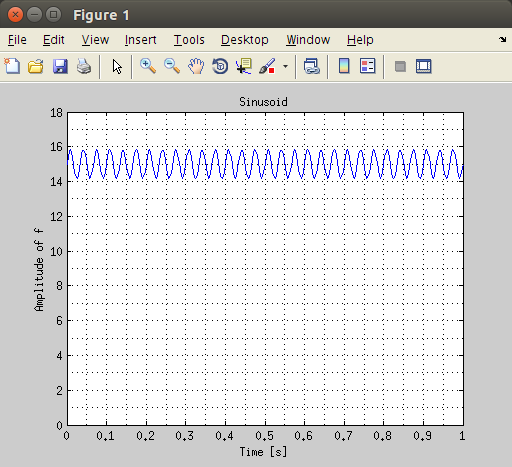
gyroscope matlab simulated
The easiest way to remove baseline is to remove the average and can be achieved with Matlab using this line!
Second Approach
Ideal situation
You will always see a slight non-zero error in the output. Now, if we analyze the frequency components of the signal we will see two elements. Please note that we are plotting only the first half of the DFT in a normalized scale. We have a peak close to zero and another one around 0.1714. To get the frequency expressed in Hz of the second component just multiply the value by the sampling rate and divide by 2. In our case:
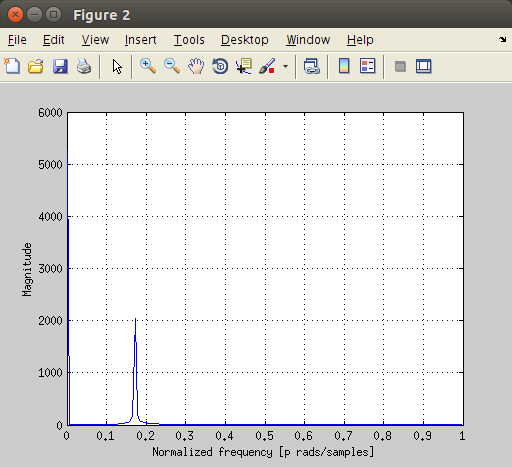
You can get the above plot with the following code.
Filter Design
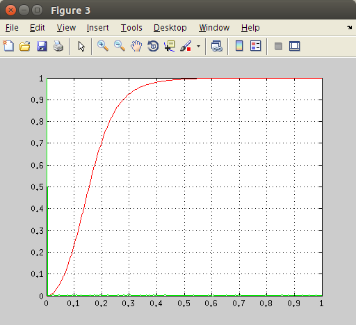
In order to suppress the low frequency component we will use a Butterworth filter with the butter function.

As we can see from the above figure, the first low frequency component is multiplied by a small gain and results attenuated (voire suppressed) and the second component is left unaffected (gain factor is 1). You can get the above figure with the following code.
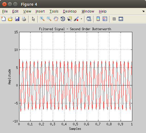
Let’s see the resutling filtered data. We expect our original sinusoid to decrease until it reaches a zero mean value.
Simulating reality
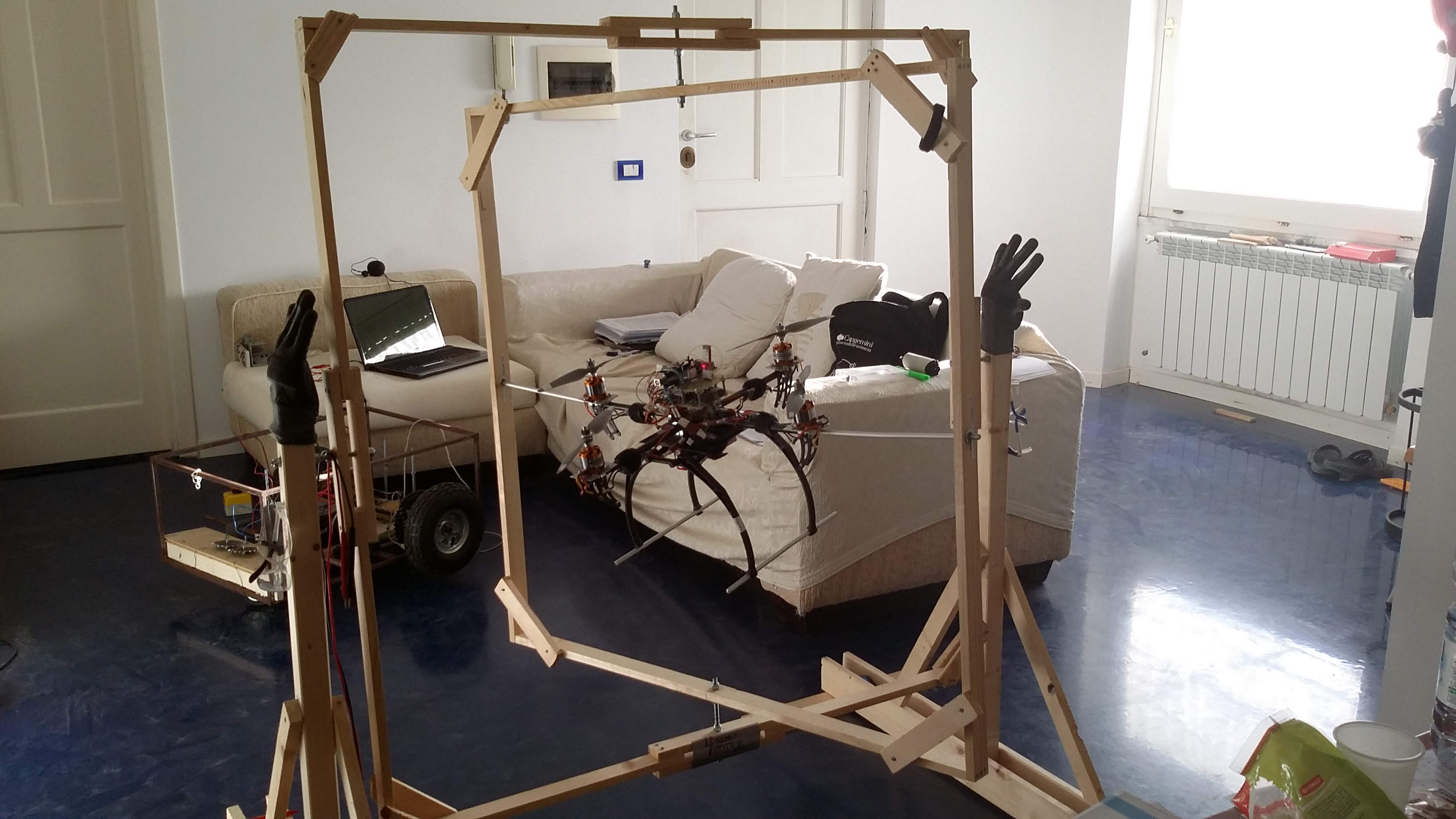
If you connect a gyroscope to your Arduino like we did in this post, you will see a small noisy signal with a DC offset. The output when the gyro is still will look like this.
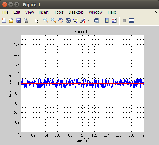
Note the DC Offset
You can use this code to obtain the blue signal.
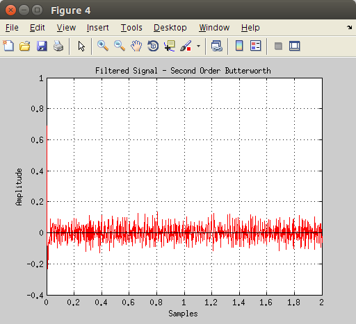
Now, let’s apply the same reasoning to this signal affected by random noise. We will use the same high pass filter with the butter function.
The resulting signal won’t be affected by the low frequency component anymore.
Full Code
Reality
What we have seen is really nice but we haven’t considered rotational movements. In this last section we will use the first approach in a real case scenario in which the gyroscope is tilted.
We will consider the .mat file available at this link.
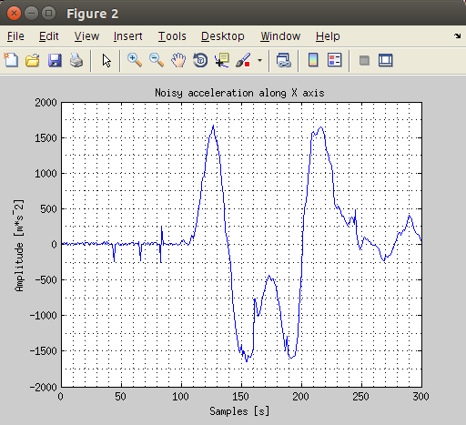
Use this code to plot data.
Now try to remove the average from data and design a high pass filter choosing a correct cutoff frequency and order.
![[ 0 ] Ubuntu instructions: Install Ubuntu Mate on Raspberry Pi 3](http://www.userk.co.uk/wp-content/uploads/2016/06/Ubuntu_MATE_GTK3-500x383.png)
![Linux Utilities and Commands 1.00 – [Quick]](http://www.userk.co.uk/wp-content/uploads/2016/01/gnu_linux_by_levhita-500x383.jpg)

![wireless network with Raspberry Pi – [Quick]](http://www.userk.co.uk/wp-content/uploads/2015/08/20150813_162509-500x383.jpg)
![Matlab Arduino – Setup a serial communication [Quick]](http://www.userk.co.uk/wp-content/uploads/2015/07/Portrait-500x383.png)