

An application of Calculus of Variation is the determination of control action $u(t)$ such that a system described by a differential equation system $$\dot{x}(t) = {a(x(t),u(t),t)}.$$ follows a trajectory $x(t)$ for all time instants that minimizes a performance measure $J(u)$ defined by
$$J(u) = \int_{t0}^{tf} {g(x(t),u(t),t)} dt$$
A wonderful application could be a tridimentional trajectory planner for quadrotor systems.
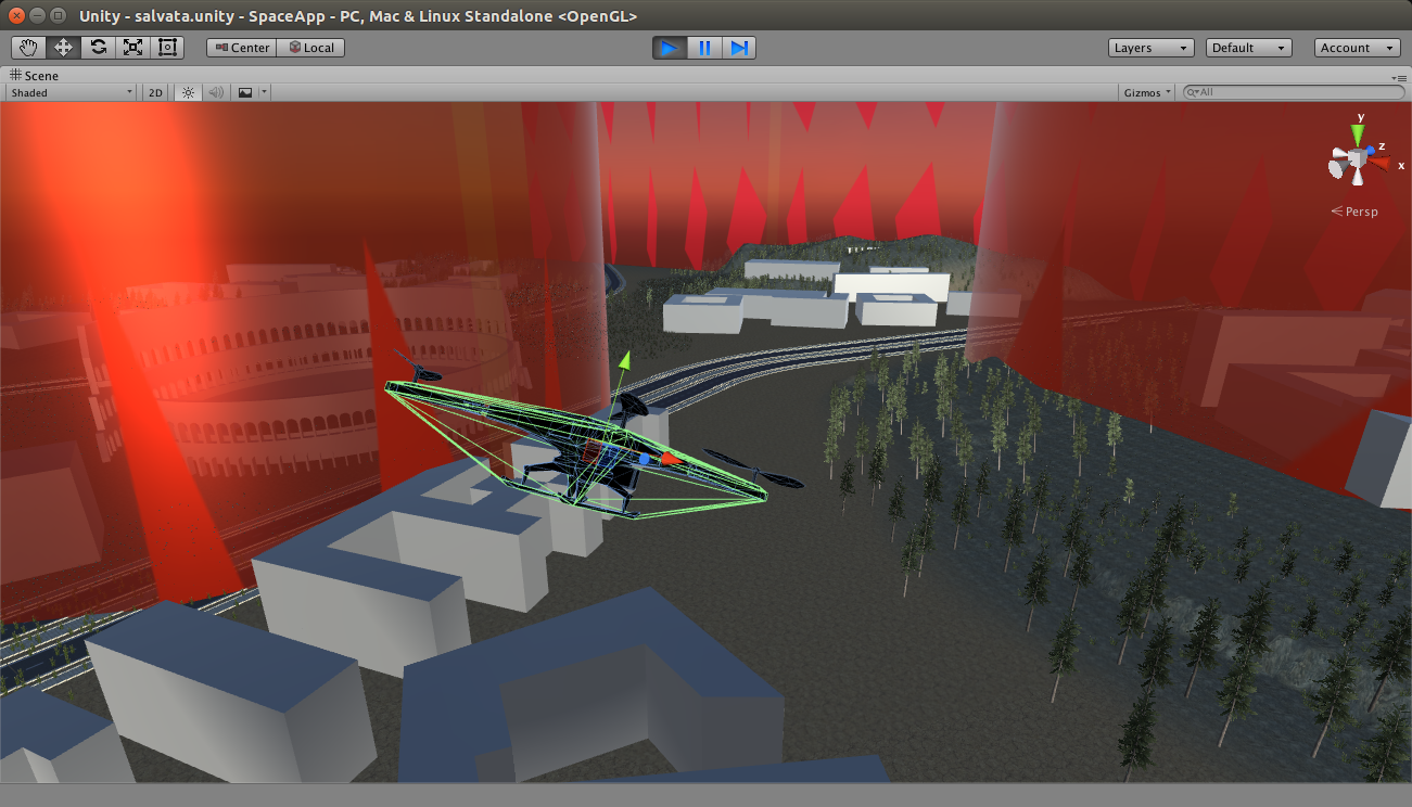
Unity 3D model
We will use the scikit-learn which is a Python module for machine learning built on top of SciPy and distributed under the 3-Clause BSD license. We will start by running the samples provided by the library then tackle the simplest problem of calculus of variation and finally we will add more complexity.
Install the Python library
Let’s start quickly by download the archive from the official website
Goto the download folder and extract the file.
userk@dopamine:~/$ cd Downloads/
userk@dopamine:~/Downloads$ ls | grep scikit
scikits.bvp_solver-1.1.tar.gz
userk@dopamine:~/Downloads$ tar xvf scikits.bvp_solver-1.1.tar.gz
userk@dopamine:~/Downloads$ ls | grep scikit
scikits.bvp_solver-1.1.tar.gz
scikits.bvp_solver-1.1
Now, build and install.
userk@dopamine:~/Downloads$ cd scikits.bvp_solver-1.1/
userk@dopamine:~/Downloads/scikits.bvp_solver-1.1$ ls
build/  MANIFEST.in  scikits/                      setup.cfg
dist/   PKG-INFO     scikits.bvp_solver.egg-info/  setup.py
userk@dopamine:~/Downloads/scikits.bvp_solver-1.1$ python setup.py build
userk@dopamine:~/Downloads/scikits.bvp_solver-1.1$ sudo python setup.py install
If you do not receive any error, you should be good to go.
First Example
Now let’s try a couple of examples from the library, for example the sample number 4 located in the scikits/bvp_solver/examples
userk@dopamine:~/Downloads/scikits.bvp_solver-1.1$ cd scikits/bvp_solver/examples
userk@dopamine:~/Downloads/scikits.bvp_solver-1.1/scikits/bvp_solver/examples$ ls
Example4.py simpleOdeBC.py TutorialExample.py
Example2.py Example5.py TemplateExample.py
Example3.py Example6.py trial.py
userk@dopamine:~/Downloads/scikits.bvp_solver-1.1/scikits/bvp_solver/examples$ python Example4.py
You should get a graph like this one.
scikits two points boundary value problem
We are not going to explore the problem tackled here.
Second Example
Now, try the example number 1. There is a wonderful documentation at this link. Here is the code we would like to run
From the documentation:
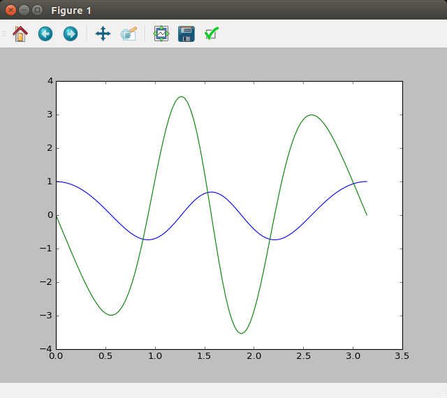
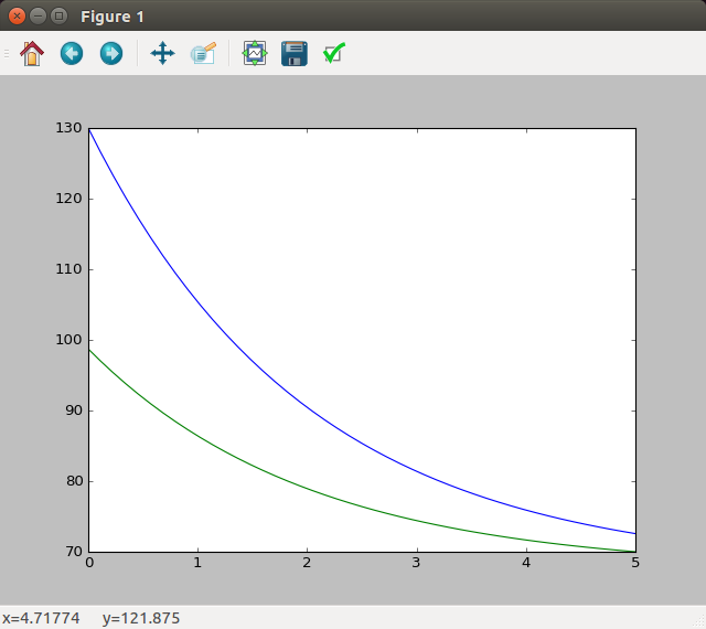
This boundary value problem describes a counter current heat exchanger; a hot liquid enters a device and exchanges heat across a metal plate with a cold liquid traveling through the device in the opposite direction. Here, T_1 is the temperature of the hot stream, T_2 is the temperature of the cold stream, q is the rate of heat transfer from the hot fluid to the cold fluid, U is the overall heat transfer coefficient and A_hx is the total area of the heat exchanger (in this case we will use 5). In this case the cold stream has twice the thermal mass of the hot stream.
Here is the graph showing the evolutions of the temperatures of the hot and cold streams T1 and T2
Ok, now that we have set up the library and run a couple of examples we can try to define a trajectory planning problem. Check the next Article